[교육봉사] 딥러닝 기초 이론

1. Neural

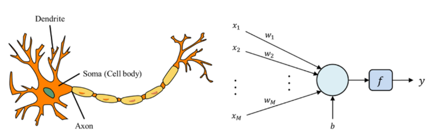
퍼셉트론은 인공신경망의 초기 형태로, 인간의 뉴런 구조를 모방하여 설계된 방식입니다. 기본적으로는 생물학적 뉴런이 전기적 신호를 받아들이고 일정 임계값을 넘어가면 다음 뉴런으로 신호를 전달하는 원리를 따르고 있습니다. 퍼셉트론에서는 각 노드가 이전 노드에서 전달받은 입력값에 가중치를 곱하여 계산하고, 이를 활성화 함수를 통해 처리한 후 다음 노드로 전달합니다.

 

이와 같은 구조는 뇌의 뉴런 간의 상호 작용을 모방함으로써 기계 학습 및 패턴 인식 등의 과제에 응용됩니다. 퍼셉트론은 입력값을 적절한 가중치와 활성화 함수를 활용하여 출력값을 생성하는데, 이를 통해 모델이 학습하고 판단할 수 있는 능력을 갖추게 됩니다. 이러한 퍼셉트론의 개념은 후에 다양한 인공신경망 모델의 기초가 되었습니다.

 

2. Perceptron

 

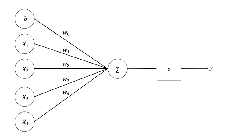
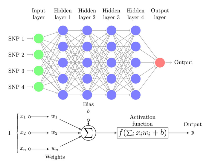
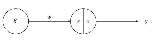
그림에서 처럼 퍼셉트론이란 생물학적인 뉴런의 특성을 모방하여서 데이터가 들어노는 input = x에 대하여 weight(가중치) 값을 곱하여 노드에 전달하고 노드에서는 activation function을 지나서 다음으로 전달하는 방식입니다.

 

Perceptron의 발전

 

X1	X2	Y
0	0	0
0	1	1
1	0	1
1	1	1

OR 연산 테이블

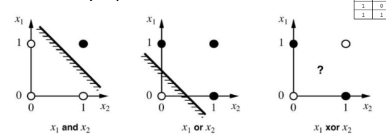
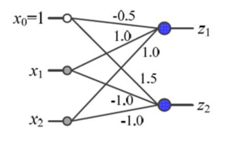
퍼셉트론의 연산을 통해서 OR, AND 게이트의 연산을 가능하게 하여서 논리적으로 연산을 통한 폭발적인 발전을 이루었다. 하지만 아래의 사진처럼 OR, AND 연산을 통한 분류는 가능했지만 XOR의 연산을 불가능하다는 한계가 발생한다. 그래서 여러 개의 Classifier를 두는 다중 퍼셉트론 구조 이론이 개발되었다.

 

 

 

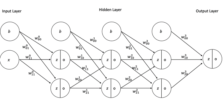
Multi-Layer perceptron

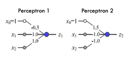
Multi-Layer Perceptron(MLP)은 기존의 Single Perceptron을 여러 개 연결하여 구성하는 인공 신경망의 한 유형입니다. Single Perceptron은 입력을 받아 가중치와 곱하고 활성화 함수를 통과한 결과를 출력하는 간단한 모델이었습니다. 그러나 Single Perceptron은 선형적인 판별 경계만을 학습할 수 있어서 비교적 간단한 문제에만 적용할 수 있었습니다.

 

 

전체 구조

 

3. Activation Function

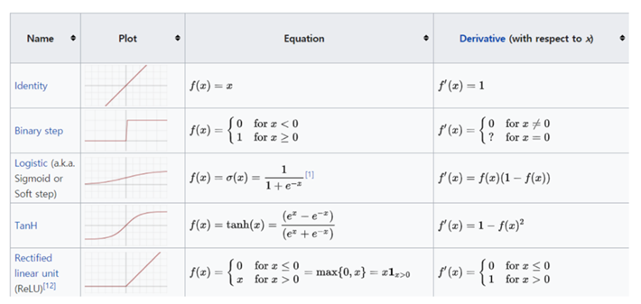
- Large derivative value : weight vanishing 문제를 해결한다.

- Easy to compute the derivate : 여러 weight 가 있는 식에서의 미분값이 아닌 활성함수의 미분

- Zero-centered : 값을 변환하여 작은 값, 양수 값으로 변환 

 

 

4. Backpropagation

 

 

import torch
import torch.nn as nn
import torch.optim as optim
from sklearn.preprocessing import LabelEncoder
from sklearn.model_selection import train_test_split
import pandas as pd
import matplotlib.pyplot as plt
import numpy as np

# Load dataset
dataframe = pd.read_csv("D:/Rworks/iris.csv")
dataset = dataframe.values
X = dataset[:, 0:4].astype(float)
Y = dataset[:, 4]

# Encode class values as integers
encoder = LabelEncoder()
encoder.fit(Y)
encoded_Y = encoder.transform(Y)

# One-hot encoding
dummy_y = pd.get_dummies(encoded_Y).values

# Divide train, test
train_X, test_X, train_y, test_y = train_test_split(X, dummy_y, test_size=0.4, random_state=321)

# Define model (DNN structure)
class SimpleModel(nn.Module):
    def __init__(self):
        super(SimpleModel, self).__init__()
        self.fc1 = nn.Linear(4, 10)
        self.relu1 = nn.ReLU()
        self.fc2 = nn.Linear(10, 10)
        self.relu2 = nn.ReLU()
        self.fc3 = nn.Linear(10, 3)
        self.softmax = nn.Softmax(dim=1)

    def forward(self, x):
        x = self.fc1(x)
        x = self.relu1(x)
        x = self.fc2(x)
        x = self.relu2(x)
        x = self.fc3(x)
        x = self.softmax(x)
        return x

model = SimpleModel()
print(model)  # Show model structure

# Define loss function and optimizer
criterion = nn.CrossEntropyLoss()
optimizer = optim.Adam(model.parameters(), lr=0.001)

# Convert data to PyTorch tensors
train_X_tensor = torch.tensor(train_X, dtype=torch.float32)
train_y_tensor = torch.argmax(torch.tensor(train_y, dtype=torch.float32), dim=1)

# Train the model
epochs = 50
batch_size = 10
disp = {'accuracy': [], 'val_accuracy': []}
for epoch in range(epochs):
    optimizer.zero_grad()
    outputs = model(train_X_tensor)
    loss = criterion(outputs, train_y_tensor)
    loss.backward()
    optimizer.step()

    # Print training statistics
    if epoch % 10 == 0:
        with torch.no_grad():
            pred = model(torch.tensor(test_X, dtype=torch.float32))
            y_classes = torch.argmax(pred, dim=1).numpy()
            accuracy = np.mean(y_classes == np.argmax(test_y, axis=1))
            disp['accuracy'].append(accuracy)
            print(f'Epoch {epoch}/{epochs} Loss: {loss.item()} Accuracy: {accuracy}')

# Plot accuracy
plt.plot(disp['accuracy'])
plt.title('model accuracy')
plt.ylabel('accuracy')
plt.xlabel('epoch')
plt.show()

# Print model weights
for name, param in model.named_parameters():
    print(name)
    print(param.data.numpy())