[교육봉사] 분류 모델 기초 이론

1.  Intro

기본적인 분류 모델에서 사용되고 있는 이론들에 대하여 정리하고 직접 실습까지 진행하는 방식으로 진행하겠습니다.

 

2. Definition

2.1 결정 트리

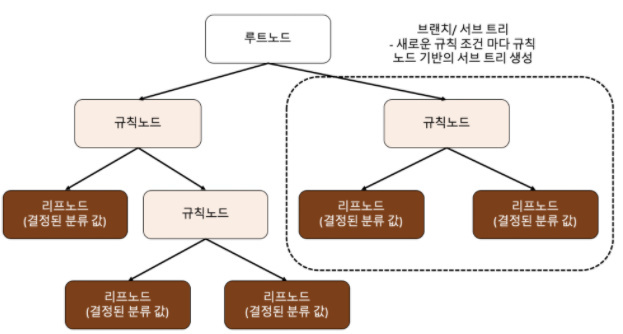
규칙 노드 : 표시된 노드는 규칙 조건이 된다.

리프 노드 : 분류된 값

서브 트리 : 전체 트리가 아닌 일부분

 

=> 하지만 트리 구조에서 깊이가 깊어질수록 결정 트리의 예측 성능이 저하될 가능성이 높다. 그래서 정확도를 높게 가지려면 최대한 많은 데이터 세트가 분류에 속하도록

 

특징으로는 직관적이라 룰이 명확하고 스케일링이나 정규화 작업이 필요하지 않는다. 하지만 결정 트리 모델의 단점은 과적합으로 정확도가 떨어진다.

 

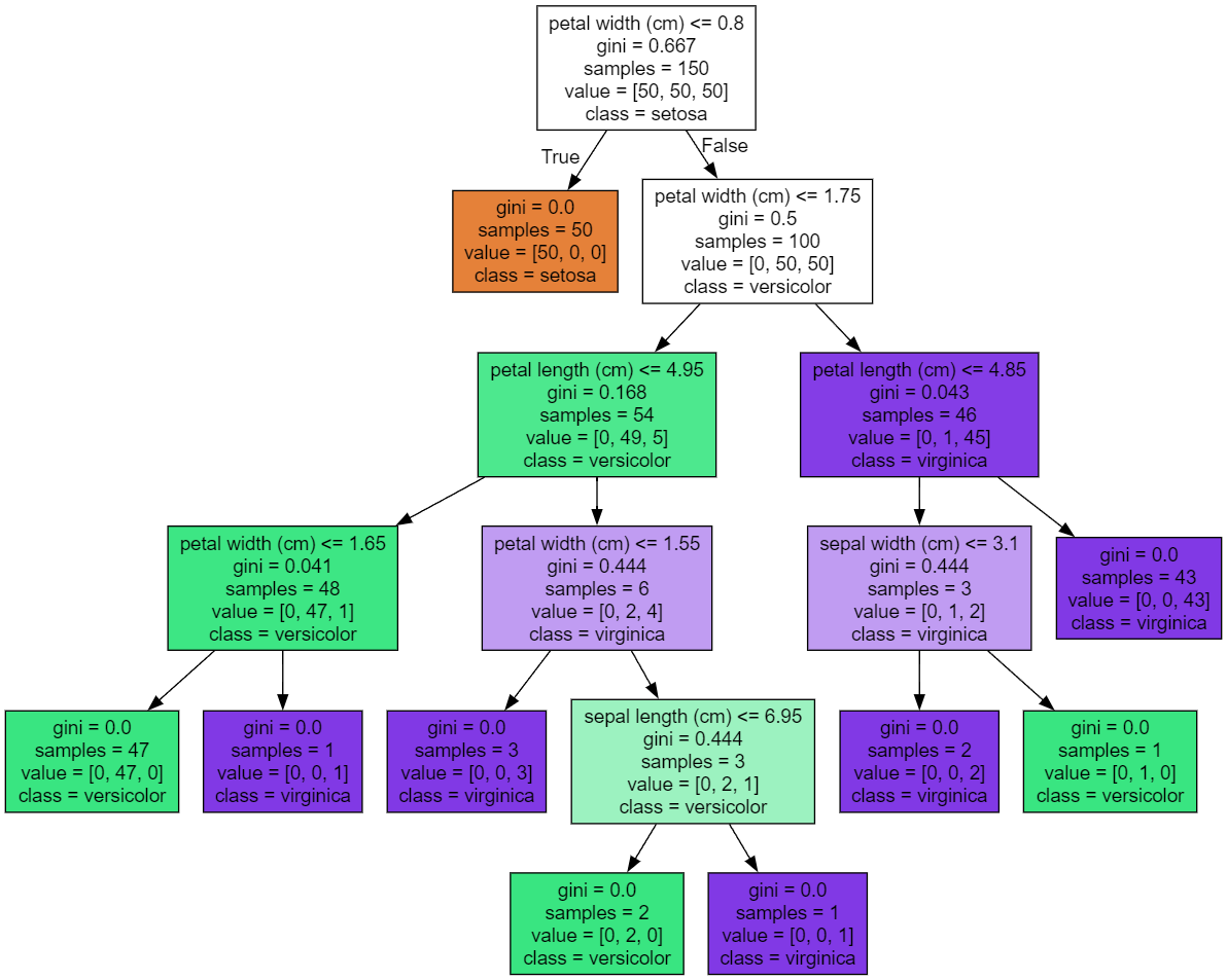
실습

from sklearn.tree import DecisionTreeClassifier, export_graphviz
from sklearn.datasets import load_iris
import graphviz

# Iris 데이터셋 로드
iris = load_iris()
X = iris.data
y = iris.target

# Decision Tree 모델 생성 및 훈련
clf = DecisionTreeClassifier()
clf.fit(X, y)

# 시각화를 위한 DOT 데이터 생성
dot_data = export_graphviz(clf, out_file="tree.dot", 
                            feature_names=iris.feature_names,  
    
                            class_names=iris.target_names,  
                            filled=True, impurity=True)

# DOT 데이터를 시각화
with open('tree.dot') as f:
    graph = f.read()

graphviz.Source(graph)

 

결과

 

 

 

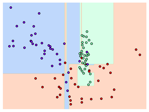
결정 트리 과적합

 

코드

import numpy as np
from sklearn.datasets import make_classification
import matplotlib.pyplot as plt
%matplotlib inline

plt.title('3 Class Values with 2 Features Sample Data Creation')

# 2차원 시각화를 위해서 피처는 2개, 클래스는 3가지 유형의 분류 샘플 데이터 생성
X_feature, y_labels = make_classification(n_features=2, n_redundant=0, n_informative=2, n_classes=3, n_clusters_per_class=1, random_state=0)

# 그래프 형태로 2개의 피처로 2차원 좌표 시각화, 각 클래스 값은 다른 색깔로 표시
plt.scatter(X_feature[:, 0], X_feature[:, 1], marker='o', c=y_labels, s=25, edgecolors='k')
# Classifier의 Decision Boundary를 시각화 하는 함수
def visualize_boundary(model, X, y):
    fig,ax = plt.subplots()
    
    # 학습 데이타 scatter plot으로 나타내기
    ax.scatter(X[:, 0], X[:, 1], c=y, s=25, cmap='rainbow', edgecolor='k',
               clim=(y.min(), y.max()), zorder=3)
    ax.axis('tight')
    ax.axis('off')
    xlim_start , xlim_end = ax.get_xlim()
    ylim_start , ylim_end = ax.get_ylim()
    
    # 호출 파라미터로 들어온 training 데이타로 model 학습 . 
    model.fit(X, y)
    # meshgrid 형태인 모든 좌표값으로 예측 수행. 
    xx, yy = np.meshgrid(np.linspace(xlim_start,xlim_end, num=200),np.linspace(ylim_start,ylim_end, num=200))
    Z = model.predict(np.c_[xx.ravel(), yy.ravel()]).reshape(xx.shape)
    
    # contourf() 를 이용하여 class boundary 를 visualization 수행. 
    n_classes = len(np.unique(y))
    contours = ax.contourf(xx, yy, Z, alpha=0.3,
                           levels=np.arange(n_classes + 1) - 0.5,
                           cmap='rainbow', clim=(y.min(), y.max()),
                           zorder=1)
dt_clf = DecisionTreeClassifier().fit(X_feature, y_labels)
visualize_boundary(dt_clf, X_feature, y_labels)

 

결과

 

 

2.2 앙상블 학습

앙상블의 기본적인 아이디어는 분류기를 여러개 사용을 하는것에 있다. 

 

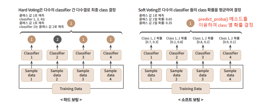
• 보팅(Voting)

하드 보팅 vs 소프트 보팅

• 배깅(Bagging)

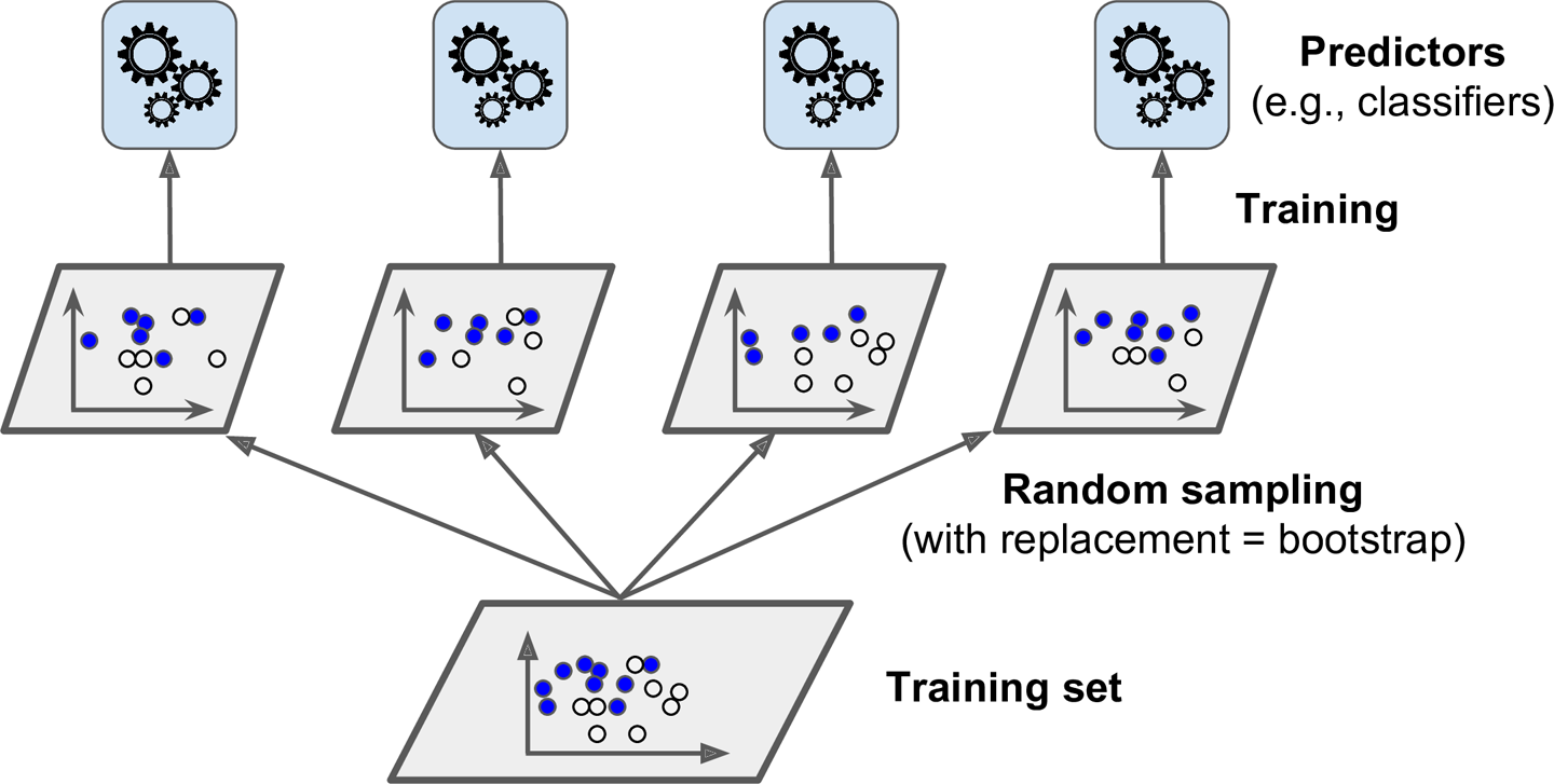
랜덤 포레스트

• 부스팅(Boosting)

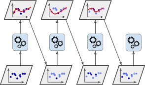
xgboost